|
This tutorial will show you how to perform discriminant analysis with Praat.
As an example, we will use the dataset from Pols et al. (1973) with the frequencies and levels of the first three formants from the 12 Dutch monophthongal vowels as spoken in /h_t/ context by 50 male speakers. This data set has been incorporated into Praat and can be called into play with the Create TableOfReal (Pols 1973)... command that can be found under New → Tables → Data sets from the literature.
In the list of objects a new TableOfReal object will appear with 6 columns and 600 rows (50 speakers × 12 vowels). The first three columns contain the formant frequencies in Hz, the last three columns contain the levels of the first three formants given in decibels below the overall sound pressure level of the measured vowel segment. Each row is labelled with a vowel label.
Pols et al. use logarithms of frequency values, we will too. Because the measurement units in the first three columns are in Hz and in the last three columns in dB, it is probably better to standardize the columns. The following script summarizes our achievements up till now:
table = Create TableOfReal (Pols 1973): "yes"
Formula: ~ if col < 4 then log10 (self) else self fi
Standardize columns
# change the column labels too, for nice plot labels.
Set column label (index): 1, "standardized log (%F__1_)"
Set column label (index): 2, "standardized log (%F__2_)"
Set column label (index): 3, "standardized log (%F__3_)"
Set column label (index): 4, "standardized %L__1_"
Set column label (index): 5, "standardized %L__2_"
Set column label (index): 6, "standardized %L__3_"
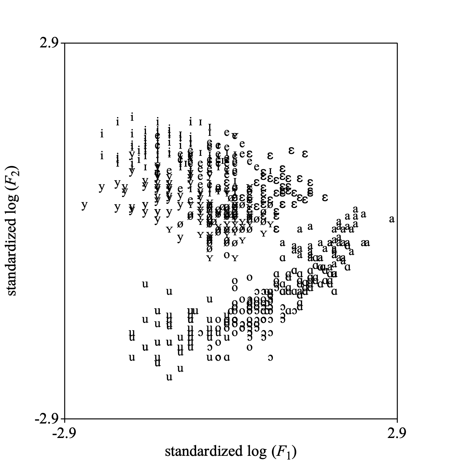
To get an indication of what these data look like, we make a scatter plot of the first standardized log-formant-frequency against the second standardized log-formant-frequency. With the next script fragment you can reproduce the following picture.
Select outer viewport: 0, 5, 0, 5
selectObject: table
Draw scatter plot: 1, 2, 0, 0, -2.9, 2.9, -2.9, 2.9, 10, "yes", "+", "yes"

Apart from a difference in scale this plot is the same as fig. 3 in the Pols et al. article.
Select the TableOfReal and choose from the dynamic menu the option To Discriminant. This command is available in the "Multivariate statistics" action button. The resulting Discriminant object will bear the same name as the TableOfReal object. The following script summarizes:
selectObject: table
discriminant = To Discriminant
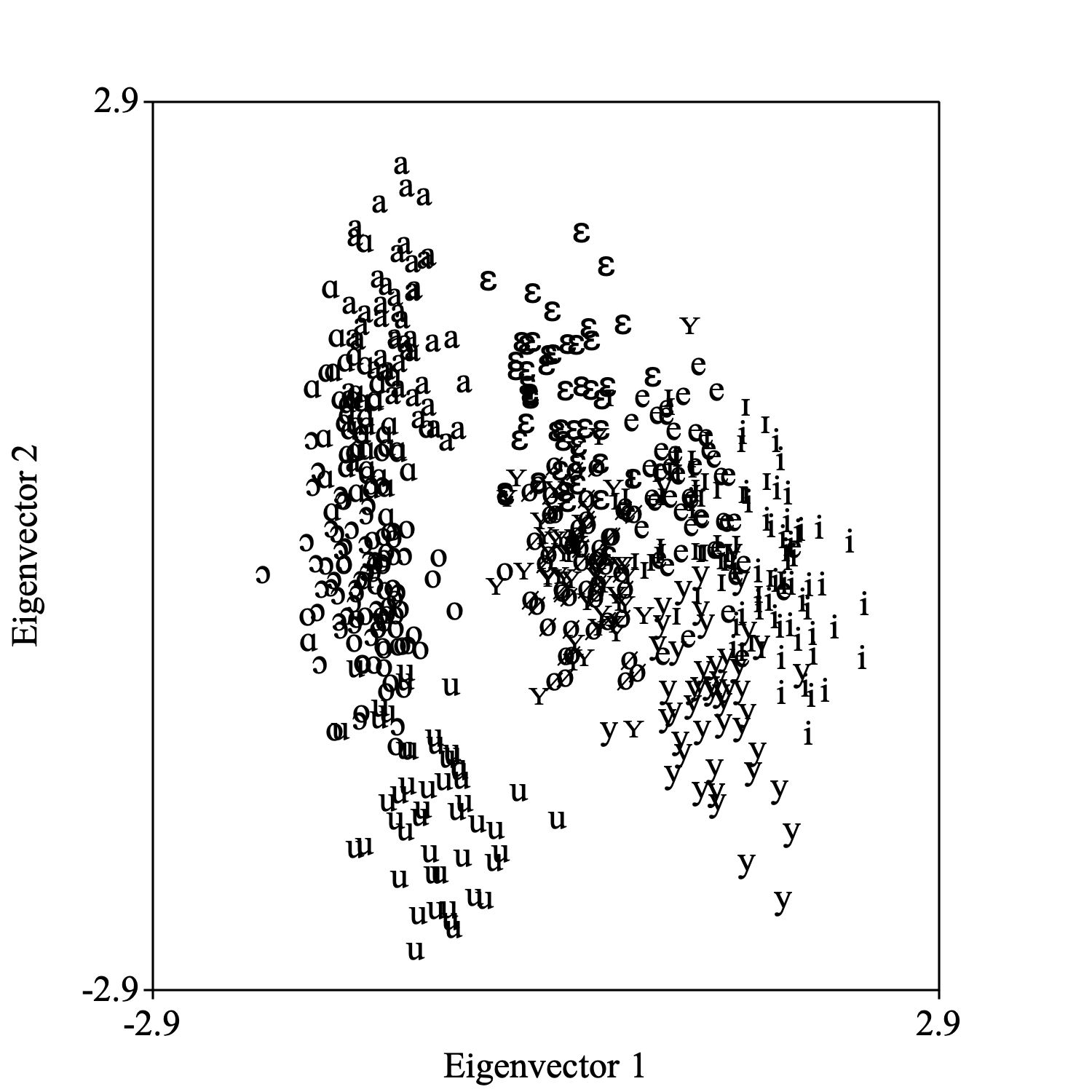
You select a TableOfReal and a Discriminant object together and choose: To Configuration.... One of the options of the newly created Configuration object is to draw it. The following picture shows how the data look in the plane spanned by the first two dimensions of this Configuration. The directions in this configuration are the eigenvectors from the Discriminant.

The following script summarizes:
selectObject: table, discriminant
To Configuration: 2
Select outer viewport: 0, 5, 0, 5
Draw: 1, 2, -2.9, 2.9, -2.9, 2.9, 12, "yes", "+", "yes"
If you are only interested in this projection, there also is a shortcut without an intermediate Discriminant object: select the TableOfReal object and choose To Configuration (lda)....
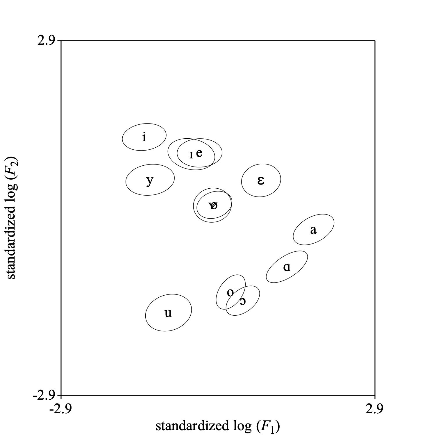
Select the Discriminant object and choose Draw sigma ellipses.... In the form you can fill out the coverage of the ellipse by way of the Number of sigmas parameter. You can also select the projection plane. The next figure shows the 1-σ concentration ellipses in the standardized log F1 vs log F2 plane. When the data are multinormally distributed, a 1-σ ellipse will cover approximately 39.3% of the data. The following code summarizes:
selectObject: discriminant
Draw sigma ellipses: 1.0, "no", 1, 2, -2.9, 2.9, -2.9, 2.9, 12, "yes"

Select together the Discriminant object (the classifier), and a TableOfReal object (the data to be classified). Next you choose To ClassificationTable. Normally you will enable the option Pool covariance matrices and the pooled covariance matrix will be used for classification.
The ClassificationTable can be converted to a Confusion object and its fraction correct can be queried with: Confusion: Get fraction correct.
In general you would separate your data into two independent sets, TRAIN and TEST. You would use TRAIN to train the discriminant classifier and TEST to test how well it classifies. Several possibilities for splitting a dataset into two sets exist. We mention the jackknife ("leave-one-out") and the bootstrap methods ("resampling").
The following script summarizes jackknife classification of the dataset:
selectObject: table
numberOfRows = Get number of rows
for irow to numberOfRows
selectObject: table
rowi = Extract rows where: ~ row = irow
selectObject: table
rest = Extract rows where: ~ row <> irow
discriminant = To Discriminant
plusObject: rowi
classification = To ClassificationTable: "yes", "yes"
if irow = 1
confusion = To Confusion: "yes"
else
plusObject: confusion
Increase confusion count
endif
removeObject: rowi, rest, discriminant, classification
endfor
selectObject: confusion
fractionCorrect = Get fraction correct
appendInfoLine: fractionCorrect, " (fraction correct, jackknifed ", numberOfRows, " times)."
removeObject: confusion
The following script summarizes bootstrap classification.
fractionCorrect = 0
for i to numberOfBootstraps
selectObject: table
resampled = To TableOfReal (bootstrap)
discriminant = To Discriminant
plusObject: resampled
classification = To ClassificationTable: "yes", "yes"
confusion = To Confusion: "yes"
fc = Get fraction correct
fractionCorrect += fc
removeObject: resampled, discriminant, classification, confusion
endfor
fractionCorrect /= numberOfBootstraps
appendInfoLine: fractionCorrect, " (fraction correct, bootstrapped ", numberOfBootstraps, " times)."
© djmw 20170829